Aruco Tag Guided Drawing Robot
Mahshid Moghadasi (mm2994)
Emmett Milliken (eam348)
December, 2020
Objective
The objective of this project was to create a mobile robot which would draw shapes on paper with the shapes input by users on a touch screen. The robot should steer using location feedback gathered using an external camera using computer vision to localize the drawing field and robot in the camera view.
Introduction
The complete code of the project can be found in the github repository:
https://github.coecis.cornell.edu/mm2994/ECE5725-Aruco-Guided-Drawing-RobotThe project is mainly based on the autonomous wheeled robot that was developed in lab 3 with an added functionality of drawing. The user would provide the input line drawing using the piTFT touchscreen. The pixel coordinates of the drawn line on the TFT will then be translated into world coordinates and the robot moves along the corresponding coordinates and leaves a trace with the marker that is attached to it. The robot gets feedback about its location from a camera that is installed on the top looking down at the robot and then decides about where to go next.
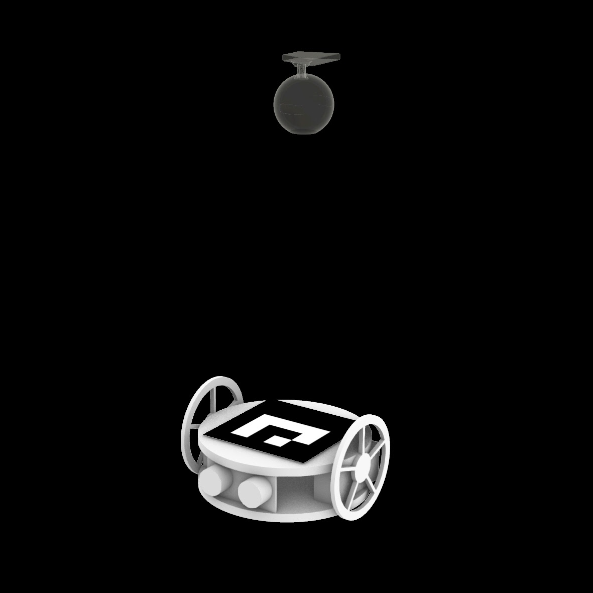
Ideation diagram, camera and the drawing robot
The project consists of the following steps:
1. Receiving input lines / points from the user on the robot-Pi
a. GUI design
2. Sending real-time pose estimation from the camera-Pi to the robot-Pi
a. Marker detection
b. Perspective correction
c. Coordinate calculation
d. Data transfer to the robot-Pi
3. Steering
a. Steering calculation

The system diagram
Design and Testing
Aruco marker detection
ArUco is an OpenSource library for detecting squared fiducial markers in images. Additionally, if the camera is calibrated, you can estimate the pose of the camera with respect to the markers.[1] We decided to use ArUco markers over April tags. ArUco markers are easier to set up, as they are already implemented in openCV library and there are fewer false detections.
Following commands are used for installing openCV on python2 and python3 respectively:
$ sudo apt-get install python-opencv
$ sudo apt-get install python3-opencv
There are several types of dictionaries within the ArUco library. We used “DICT_4X4_50” and used the code below to generate a set of fifty 4 by 4 pixel markers, based on the documentation linked below:
Import cv2
import numpy as np
import cv2.aruco as aruco


# Load the predefined dictionary
dictionary = cv2.aruco.Dictionary_get(cv2.aruco.DICT_4X4_50) #size is 4 by 4 and number is 50 - faster


def aruco_create():
   for i in range(50):
       # Generate the markers
       outputMarker = np.zeros((200, 200), dtype=np.uint8)
       markerImage = cv2.aruco.drawMarker(dictionary, i, 500, outputMarker, 1) #500 is the number of pixels
       image_path = r'/home/pi/project/aruco/4X4Marker%i.jpg' %i
       cv2.imwrite(image_path , markerImage)


aruco_create()
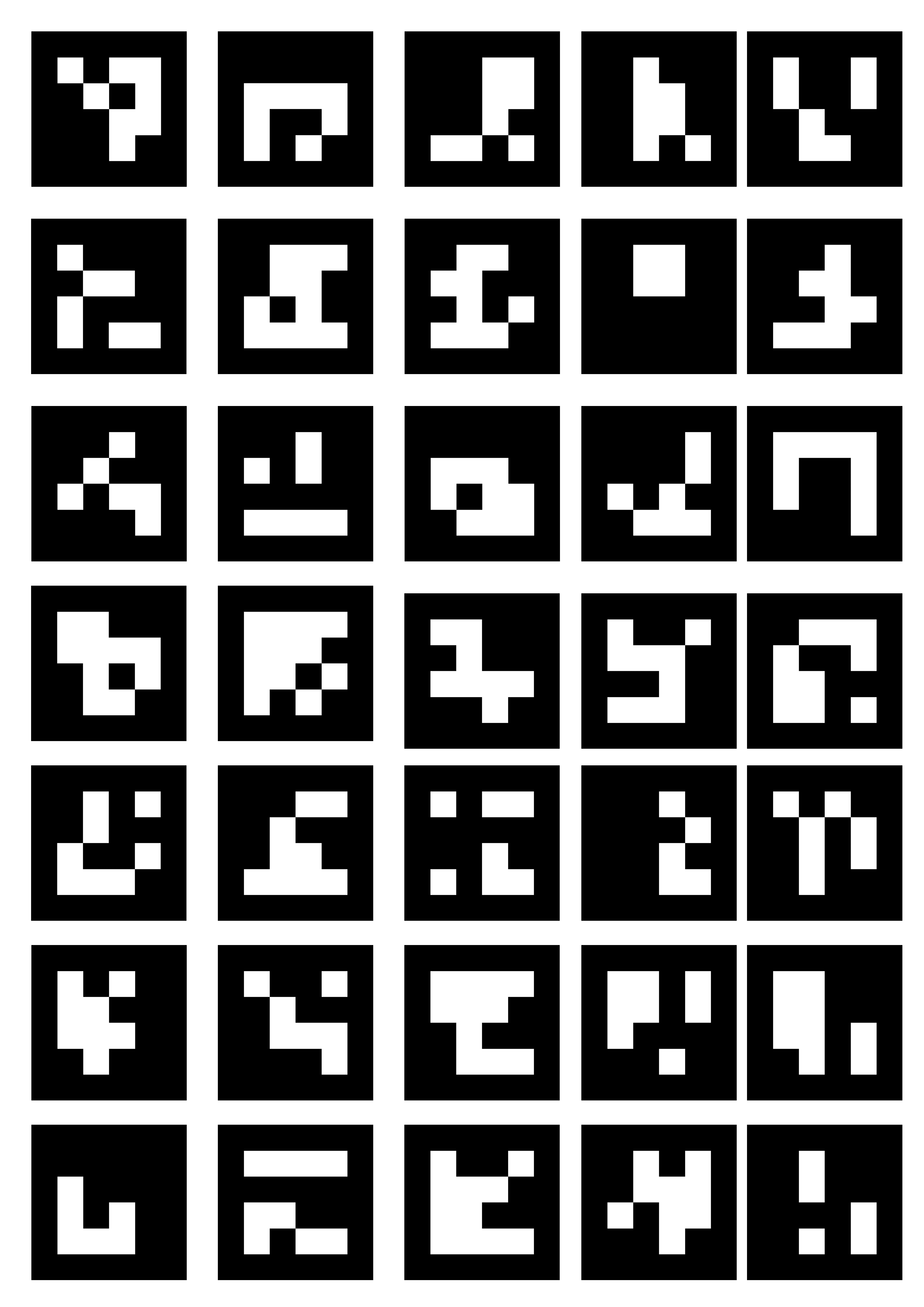
left: ArUco dictionary 50_4X4
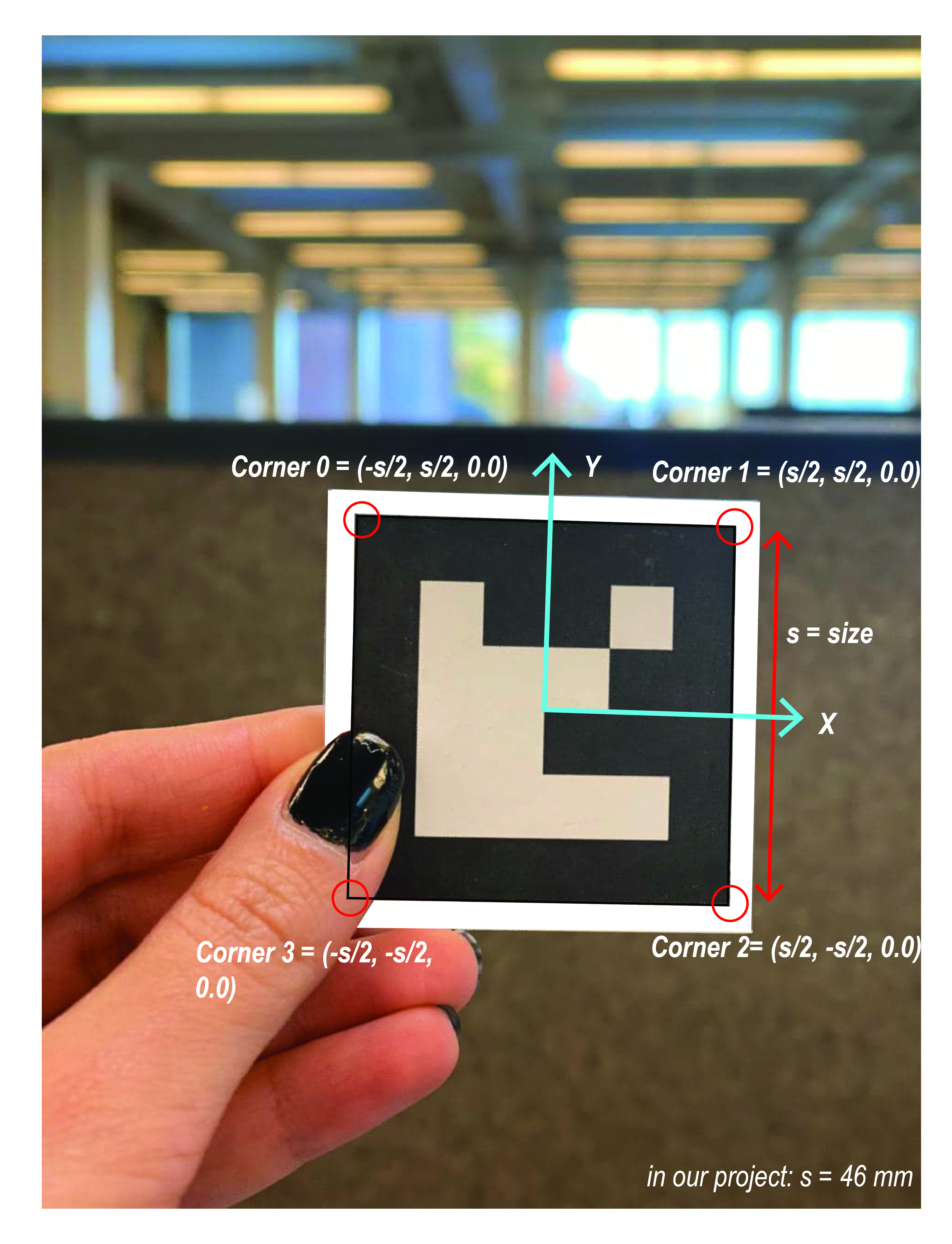
right: ArUco marker #32 corners and orientation from 50_4X4 dictionary
After printing the markers, we used the following code to detect the markers. It is important to note that there should be a white offsetted background around the markers for the true detection. Corners of the markers are stored in a list based on the order shown in the photo:
0: top left corner
1: top right corner
2: bottom right corner
3: bottom left corner
This is important because the perspective correction calculations and robot pose estimation, specifically the direction of the robot are based on the corners and the orientation of the marker. Many errors can occur simply because of lack of attention to the correct positioning of the marker.
Import cv2
import numpy as np
import cv2.aruco as aruco

#Aruco detection
cap = cv2.VideoCapture(0)

while True:
   ret, frame = cap.read()
   gray = cv2.cvtColor(frame, cv2.COLOR_BGR2GRAY)

   aruco_dict = aruco.Dictionary_get(aruco.DICT_4X4_50)
   arucoParameters = aruco.DetectorParameters_create()
   corners, ids, rejectedImgPoints = aruco.detectMarkers(
       gray, aruco_dict, parameters=arucoParameters)
   print(ids)
   if np.all(ids):
     image = aruco.drawDetectedMarkers(frame,corners,ids)
     cv2.imshow('Display', image)
   else:
       display = frame
       cv2.imshow('Display', display)

   if cv2.waitKey(1) & 0xFF == ord('q'):
       break

cap.release()
cv2.destroyAllWindows()

ArUco marker detection with their corresponding orientation and rotation
Camera calibration
Geometric Camera calibration, also known as camera resectioning, estimates the parameters of the camera. This includes the intrinsic parameters of the lens, the extrinsic parameters of the camera and its distortion coefficients. These parameters are required for machine vision applications, such as calculating the position and dimensions of an object in the real world. For calibrating any camera, we need to have 3D world points and their corresponding 2D image points of a known object or pattern. [2] We calibrated the Pi Camera based on the classical openCV chessboard [3]:
We printed the chessboard below and attached it on a stiff board. Once printed we used the code below to take photos of the board from different angles and perspectives every 2 seconds and save them to the directory. For the best result, at least 15 photos are required.
import cv2
import numpy as np
import cv2.aruco as aruco
import time
cap = cv2.VideoCapture(0)
last_recorded_time = time.time()
frame_count = 0

while True:
 _, frame = cap.read()
 curr_time = time.time()
 cv2.imshow('Display', frame)
 if (curr_time - last_recorded_time >= 2.0):
   cv2.imwrite('frame_{}.png'.format(frame_count), frame)
   last_recorded_time = curr_time
   frame_count+=1
 if cv2.waitKey(1) & 0xFF == ord('q'):
   break

cap.release()
cv2.destroyAllWindows()
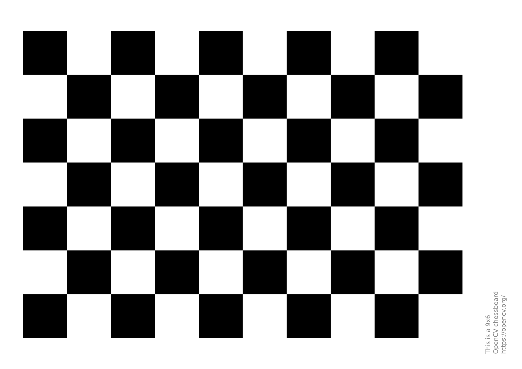
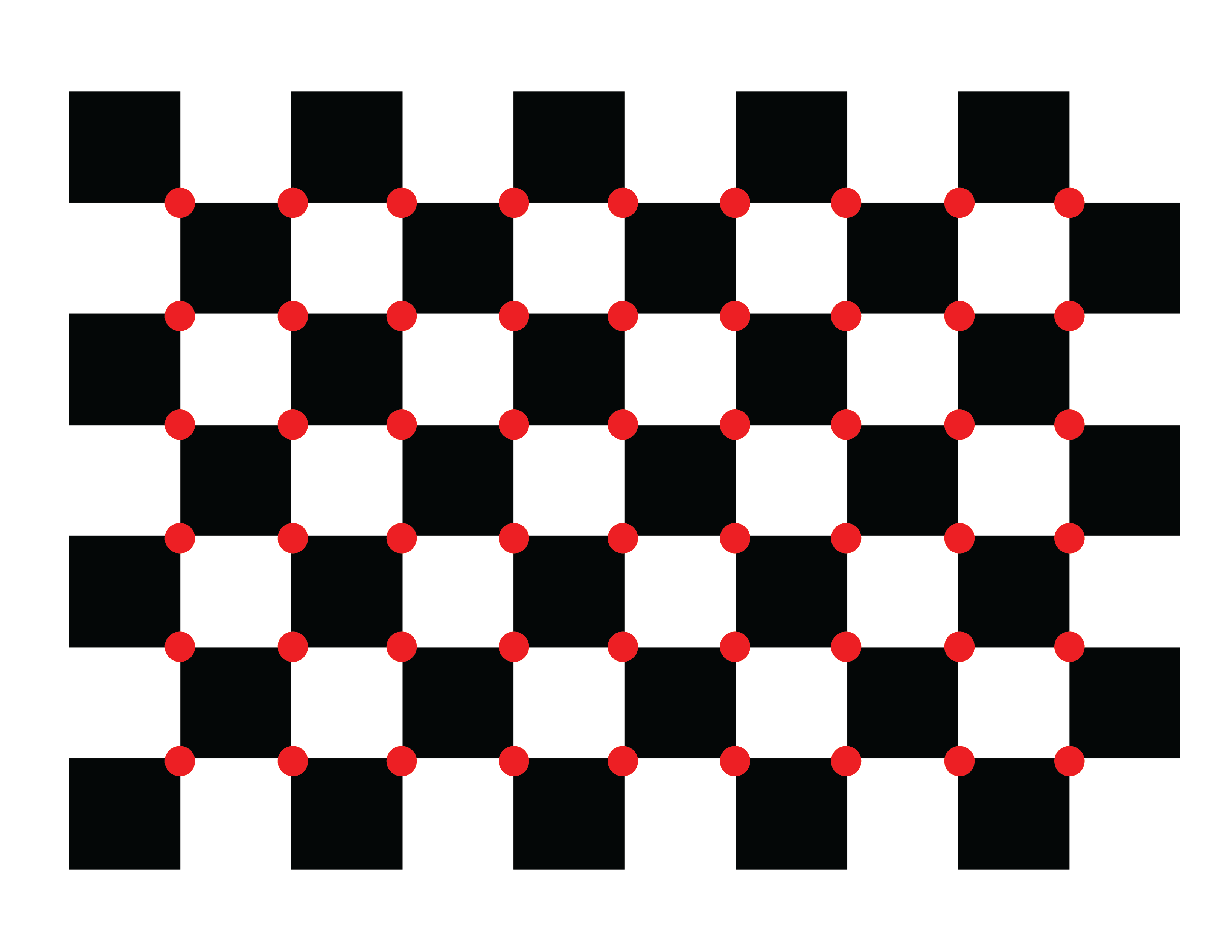
left: OpenCV chessboard
right: 6 by 9 grid of interior points as inputs for the camera calibration code
Then we used the photos taken in the previous step and basic measurements of the chessboard to calibrate the camera:
1) square size: 0.035 meters
2) number of points inside the grid in each row and column: 6 by 9 - It’s important to know that this is the number of points inside the grid as shown in the photo above and not the number of squares.
import numpy as np
import cv2
import glob

# termination criteria
criteria = (cv2.TERM_CRITERIA_EPS + cv2.TERM_CRITERIA_MAX_ITER, 30, 0.001)

# prepare object points, like (0,0,0), (1,0,0), (2,0,0) ....,(6,5,0)
# size of each square is 35 mm
square_size = 0.0355 #in meters
objp = np.zeros((6*9,3), np.float32)
objp[:,:2] = (square_size * np.mgrid[0:9,0:6]).T.reshape(-1,2)

# Arrays to store object points and image points from all the images.
objpoints = [] # 3d point in real world space
imgpoints = [] # 2d points in image plane.

images = glob.glob(r'/home/pi/project/calib_photos/*.png',)

for fname in images:
   img = cv2.imread(fname)
   gray = cv2.cvtColor(img,cv2.COLOR_BGR2GRAY)
   sample_im = gray
   #cv2.imshow(gray)
   # Find the chess board corners
   chessboard_flags = cv2.CALIB_CB_ADAPTIVE_THRESH + cv2.CALIB_CB_NORMALIZE_IMAGE
   flags = 0
   flags |= cv2.CALIB_CB_ADAPTIVE_THRESH
   flags |= cv2.CALIB_CB_NORMALIZE_IMAGE
   [ret, corners] = cv2.findChessboardCorners(gray, (9, 6), flags)

   # If found, add object points, image points (after refining them)
   if (ret == True):
       #print ('True')
       objpoints.append(objp)
       corners2 = cv2.cornerSubPix(gray,corners,(11,11),(-1,-1),criteria)
       imgpoints.append(corners2) #these are the found corners

       # Draw and display the corners
       img = cv2.drawChessboardCorners(img, (9,6), corners2,ret)
       cv2.imshow('img',img)
       cv2.waitKey(100)

cv2.destroyAllWindows()
ret, mtx, dist, rvecs, tvecs = cv2.calibrateCamera(objpoints, imgpoints, gray.shape[::-1], None, None)


# Undistortion
# refine the camera matrix
ii = -1
for fname in images:
   #if (fname==images[0]):
   ii +=1
   img = cv2.imread(fname)
   h,  w = img.shape[:2]
   newcameramtx, roi=cv2.getOptimalNewCameraMatrix(mtx,dist,(w,h),1,(w,h))
   dst1 = cv2.undistort(img, newcameramtx, dist, None, None)

   # testing if the matrix is right
   image_path1 = r'/home/pi/project/calib_photos/final/%i.png' % ii
   cv2.imwrite(image_path1, dst1)

path = r'/home/pi/project/picamera.yml'
cv_file = cv2.FileStorage(path, cv2.FILE_STORAGE_WRITE)
cv_file.write("new_matrix", newcameramtx)
cv_file.write("distortion_coef", dist)

cv_file.release()

# Re-projection Error
tot_error = 0
for i in range(len(objpoints)):
   imgpoints2, _ = cv2.projectPoints(objpoints[i], rvecs[i], tvecs[i], mtx, dist)
   error = cv2.norm(imgpoints[i],imgpoints2, cv2.NORM_L2)/len(imgpoints2)
   tot_error += error

print ("total error: ", tot_error/len(objpoints))
Photos below show the true detection of the aforementioned points:

Sample input photos for camera calibration - the algorithm has successfully detected the interior point grid
%YAML:1.0
---
new_matrix: !!opencv-matrix
  rows: 3
  cols: 3
  dt: d
  data: [ 5.0729638671875000e+02, 0., 3.1174656415419304e+02, 0.,
      5.0761346435546875e+02, 2.3997776397076632e+02, 0., 0., 1. ]
distortion_coef: !!opencv-matrix
  rows: 1
  cols: 5
  dt: d
  data: [ 1.9076841407258338e-01, -4.5190192083740538e-01,
      2.7079765950399783e-04, 1.3991690924355539e-04,
      2.7966157704609523e-01 ]
Once the calibration was completed, we calculated the projection error to evaluate the accuracy of the estimated parameters.
Finally the camera parameters are stored in a .yaml file. We will later load the file in the final code and use the camera parameters for accurate pose estimation.
Camera perspective correction
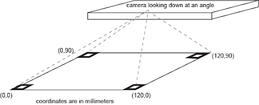
Any two images of the same planar surface in space are related by a homography. [4] If we know the coordinates of four predefined points in each surface plane, we will be able to calculate the homography / projection matrix. Therefore we will be able to calculate the coordinates of any given point in either of the planes using its corresponding coordinate in the other plane. Matrix H in the equation below is the homography matrix. [5]

Implementing homography matrix for perspective correction
We used the same logic to correct the perspective transformation in the pi Camera image. Four ArUco markers are placed at the corners of the space that the robot will operate in. The distance between the markers, i.e. the length and width of the area is measured and stored in variables worldx and worldy. The markers which are placed in each corner, as well as the marker on the robot and their size are defined as well.
We set the marker placed at the bottom left to be the origin and considered the right direction from the origin as +x and the top direction as +y. Therefore the robot space is described as :
[0.0, 0.0], [worldx, 0.0], [0.0, worldy], [worldx, worldy]
The code detects the markers, and using the aforementioned information calculates the homography matrix. The homography matrix corrects the perspective transformation and calculates the real-world coordinate of any point within the defined space, including the position of the robot.

Implementing homography matrix for perspective correction
import socket
import cv2
import numpy as np
import datetime
import cv2.aruco as aruco
import glob
import math
import faulthandler; faulthandler.enable()
import multiprocessing as mp
import time

#IP = '192.168.0.246' #Emmett’s Robot IP
IP = '192.168.137.120' #Mahshid's Robot IP
port = 5000
marker_dimension = 0.046  #4.6 centimeter before
worldx = 889 #508#-marker_dimension*1000 #millimeters
worldy = 508 #401#-marker_dimension*1000 #millimeters
# modify these based on your enviornment settings
robot_ID = 7
bottom_left = 31  #this is the origin - positivex: towards bottom right - positivey: towards top left
bottom_right = 32
top_left = 9
top_right = 20

def UDP(IP,port,message):
   sock = socket.socket(socket.AF_INET, socket.SOCK_DGRAM) #IPv4 DNS server - UDP protocol
   sock.sendto(bytes(message, "utf-8"), (IP,port)) #self, data, address

def getMarkerCenter(corners):
 px = (corners[0][0] + corners[1][0] + corners[2][0]+ corners[3][0]) * 0.25
 py = (corners[0][1] + corners[1][1] + corners[2][1]+ corners[3][1]) * 0.25
 return [px,py]

def getMarkerRotation(corners):
 unit_x_axis = [1.,0.]
 center = getMarkerCenter(corners)
 right_edge_midpoint = (corners[1]+corners[2])/2.
 unit_vec = (right_edge_midpoint-center)/np.linalg.norm(right_edge_midpoint-center)
 angle = np.arccos(np.dot(unit_x_axis,unit_vec))
 return angle

def inversePerspective(rvec, tvec):
   R, _ = cv2.Rodrigues(rvec)
   R = np.array(R).T #this was np.matrix but had error
   invTvec = np.dot(-R, np.array(tvec))
   invRvec, _ = cv2.Rodrigues(R)
   return invRvec, invTvec
def normalize(v):
   if np.linalg.norm(v) == 0 : return v
   return v / np.linalg.norm(v)

"""" the function gets the corners of an aruco marker in the camera space as the origin with its
X (Green) and Y (Red) axis. The origin is the bottom left corner, the coordinate of the point is calculated
in relation to this origin """
def findWorldCoordinate(originCorners, point):
   zero = np.array(originCorners[3]) #bottom left as the origin - check the data structure
   x = (np.array(originCorners[0]) - zero)  # bottom right - Green Axis -- throw out z
   y = (np.array(originCorners[1]) - zero)   # top left - Red Axis -- throw out z
   x = x[0][0:2]
   y = y[0][0:2]
   x = normalize(x)
   y = normalize(y)
   #print("x", x)
   vec = (point - zero)[0][0:2]
   #print("vec", vec)
   vecNormal = normalize(vec)
   cosX = np.dot(x,vecNormal)
   cosY = np.dot(y,vecNormal)
   xW = np.linalg.norm(vec) * cosX
   yW = np.linalg.norm(vec) * cosY
   return [xW, yW]
################################
try:
   # Getting the camera calibration information
   path = r'/home/pi/ECE-5725/camera_codes/picamera.yml'
   cv_file = cv2.FileStorage(path, cv2.FILE_STORAGE_READ)
   new_matrix = cv_file.getNode("new_matrix").mat()
   dist_matrix = cv_file.getNode("distortion_coef").mat()
   mtx = cv_file.getNode("matrix").mat()
   cv_file.release()

   found_dict_pixel_space = {}
   found_dict_camera_space = {}
   found_dict_world_space = {}
   found_dict_homography_space = {}
   final_string = ""
   originRvec = np.array([0,0,1])
   markerRvec= np.array([0,0,0])

 # read aruco markers and create dictionary
   aruco_source_path = glob.glob(r'/home/pi/ECE-5725/camera_codes/aruco/*.jpg', )
   aruco_source = []
   for ar in aruco_source_path:
       im_src = cv2.imread(ar)
       aruco_source.append(im_src)
   aruco_dict = aruco.Dictionary_get(aruco.DICT_4X4_50)

   cap = cv2.VideoCapture(0)
   #pool = mp.Pool(mp.cpu_count()) # init pool for multiprocessing

   while True:
       t0 = time.time()
       #ret, frame = cap.read() # read frame
       ret, image = cap.read() # read frame
       #cv2.imshow('frame', frame)
       t1 = time.time()-t0
       #----aruco detection-------------------
       gray = cv2.cvtColor(image, cv2.COLOR_BGR2GRAY) # converts image color space from BRG to grayscale
       t2 = time.time()-t0
       data = aruco.detectMarkers(gray, aruco_dict) # detect aruco markers

       t3 = time.time()-t0
       corners = data[0] # corners of found aruco markers
       ids = data[1] # ids of found aruco markers
       originIDglobal = 0
       if np.all(ids): # if any markers were found
           #print("found one!")
           t4 = time.time()-t0
           result = aruco.estimatePoseSingleMarkers(corners, marker_dimension, new_matrix, dist_matrix) # estimate the pose of the markers
           rvecs = result[0] # rotation vectors of markers
           tvecs = result[1] # translation vector of markers
           imageCopy = image

           #setting bottom_left as the origin
           if bottom_left in ids:
               originID = np.where(ids == bottom_left)[0][0]
               originIDglobal = originID
           else:
               originID = originIDglobal
           originCorners = corners[originID] # corners of the tag set as the origin
           OriginCornersCamera = getCornerInCameraWorld(marker_dimension, rvecs[originID], tvecs[originID])[0] # origin tag corners in camera space
           originRvec = rvecs[originID] # rotation vec of origin tag
           originTvec = tvecs[originID] # translation vec of origin tag

           display = cv2.aruco.drawDetectedMarkers(imageCopy,corners,ids) # display is image copy with boxes drawn around the tags
           t5 = time.time()-t0
           for i in range(len(ids)): # for each tag found in image
               ID = ids[i]
               rvec = rvecs[i]
               tvec = tvecs[i]
               corners4 = corners[i]

               display = cv2.aruco.drawAxis(imageCopy,new_matrix,dist_matrix,rvec,tvec,0.03) # draw 3d axis, 3 centimeters
               found_dict_pixel_space[""+str(ids[i][0])] = corners4 # put the corners of this tag in the dictionary

           # Homography
           zero = found_dict_pixel_space[str(bottom_left)][0][3] #bottom left - 3
           x = found_dict_pixel_space[str(bottom_right)][0][2] #bottom right - 27
           y = found_dict_pixel_space[str(top_left)][0][0] #top left - 22
           xy = found_dict_pixel_space[str(top_right)][0][1] #top right - 24

           workspace_world_corners = np.array([[0.0, 0.0], [worldx, 0.0], [0.0, worldy], [worldx, worldy]], np.float32) # 4 corners in millimeters
           workspace_pixel_corners = np.array([zero,x,y,xy], np.float32)  # 4 corners in pixels

           # Homography Matrix
           h, status = cv2.findHomography(workspace_pixel_corners, workspace_world_corners) #perspective matrix
           t6=time.time()-t0
           im_out = cv2.warpPerspective(image, h, (worldx,worldy)) #showing that it works

           t7 = time.time()-t0
           for i in range(len(ids)):
               j = ids[i][0]
               corners_pix = found_dict_pixel_space[str(j)]#[0]
               corners_pix_transformed = cv2.perspectiveTransform(corners_pix,h)
               found_dict_homography_space[str(j)] = corners_pix_transformed
           print(found_dict_homography_space)
           robot = found_dict_homography_space[str(robot_ID)][0]
           print(getMarkerCenter(robot))
           cv2.imshow('Warped Source Image', im_out)
           t8=time.time()-t0
           print("t1: %8.4f   t2: %8.4f   t3: %8.4f   t4: %8.4f   t5: %8.4f   t6: %8.4f   t7: %8.4f   t8: %8.4f" %(t1,t2-t1,t3-t2,t4-t3,t5-t4,t6-t5,t7-t6,t8-t7))

       else:
           display = image
           cv2.imshow('Display', display)

       ###### sending the data to the robot ########################
       robot_center = getMarkerCenter(robot)
       robot_angle = getMarkerRotation(robot)
       #UDP(IP, port, str([robot_center[0], robot_center[1],robot_angle,worldx,worldy]))
       UDP(IP, port, str([robot_center[0], robot_center[1], robot[1][0], robot[1][1], robot[0][0], robot[0][1], worldx, worldy]))

       if cv2.waitKey(1) & 0xFF == ord('q'):
           break

except Exception as e:
 print(e)

# When everything done, release the capture
cap.release()
cv2.destroyAllWindows()
UDP connection between the Pi's
We needed to have some form of communication between the camera and the robot in order to aid in robot localization. A UDP connection was chosen for this connection because our priorities were simplicity and minimal update delay, and the system is tolerant of individual packet loss. UDP has the advantage over TCP in this situation in that UDP does not require an established connection, which simplifies operation of the system. The camera can continuously send the coordinates of the robot Aruco tag without waiting for acknowledgements from the robot or waiting to establish a connection. This allowed the camera code to be started once and left running uninterrupted for multiple runs of the robot code. The camera not needing to wait for acknowledgments as it would with TCP also reduced the time between updates sent to the robot. This system is tolerant to packet loss because only the most up-to-date robot location is used in the robot steering, which means there is no point in retransmitting older data if it were to get lost. The camera Pi is set up as a UDP client and the robot Pi as a UDP server.
# get current robot coords from camera
  raw_data, address = s.recvfrom(4096)
  #print("\n\n 2. Server received: ", data.decode('utf-8'), "\n\n")
  data=raw_data.decode('utf-8')
  data = data[1:-1]
  data = data.split(',')

  center_x, center_y,right_x,right_y,left_x,left_y,world_x, world_y  = map(float,data) #UDP data

Camera sends the coordinate information to the robot through UDP communication
Touchscreen GUI
Drawing shapes from user input requires having a way for users to provide those shapes. We chose to use a very simple graphical user interface (GUI) on a touchscreen mounted to the top of the drawing robot. The GUI consists of a white background with three buttons at the bottom of the touchscreen. These three buttons are "clear", "done", and "quit". Users can draw the shapes they wish for the robot to replicate on the white background of the screen. There is no functional limit on the number of lines which a user can input.
With our setup, touchscreen events register as mouse events. Events for when a mouse click is started, the mouse moves, and a mouse click is released are the events used by our GUI. When a mouse click is started we first check if the mouse is within the area of any of our buttons. If the touch is not in the area of the buttons, then a new line is started. A new point is added to the line at each successive mouse move event until a mouse release is detected. Once the release is detected, the line is added to the list of lines which have been drawn. The clear button can be used to erase all of the lines currently recorded. The done button allows the user to finalize the set of drawn lines and start the process of the robot drawing the lines. The clear and done buttons disappear after the done button has been pressed. The quit button can be used at any point in the program to immediately stop the robot and safely exit the program.

Graphic User Interface - left button: clear - middle button: done - right button: quit
Pen lifter
We needed something that would allow our robot to hold a pen so that it could draw. In order to draw lines only in the desired location rather than every place the robot moves, we needed to be able to raise and lower the pen. This project is not focused on 3D design, and a servo controlled pen is not a totally novel idea, so we looked for options on Thingiverse. One of the most fun designs we came across was for the Sphere-O-Bot/Eggbot, which will draw designs on a small sphere or an egg. [6] The arm holding the pen/marker used the same type of servo that we were using, and the form factor seemed to fit our application, so we decided to use this design in our robot. Some modifications were used for different pen sizes.
The pen is lightweight and the movement to raise and lower the pen does not need great precision, so we were able to use inexpensive servos which both partners just had laying around. Both partners had knock-off versions of the Tower Pro SG90 servo. [7] These servos required separate control functions from those used to control our drive servos. The SG90 communication protocol requires PWM signal with a period of 20 ms, with high times ranging from 1 ms to 2 ms, with 1 ms corresponding to -90 degrees, 1.5 ms to 0 degrees, and 2 ms to +90 degrees. This pen lifting servo is powered off of a separate set of batteries from the Raspberry Pi.

3400 robot with the marker attachment
Robot servos
The robot we used is referred to as the "ECE 3400" robot, due a similar robot base being used in that class. This robot uses two Parallax continuous rotation servos [8] to power the drive wheels at the front of the robot, and a small ball bearing as a caster to hold up the back.
While the Tower Pro servo communication uses a 20 ms period, the Parallax servo communication requires 20 ms low time. The speed and direction of the servo is controlled by the high time of the PWM signal, with a range of 1.3 ms to 1.7 ms. 1.3 ms is full speed in the clockwise direction, 1.5 ms to not moving, and 1.7 ms to full speed counter-clockwise. The 20 ms low time with a variable high time results in a PWM signal which must change frequency as well as duty cycle in order to change the speed and/or direction of the servo.
In order for the two servos to spin at similar speeds when the same logic value is applied, they must be calibrated. This is done by sending a signal with a 1.5 ms high time to the servos and using a small screwdriver to adjust the calibration screw until the servos do not move.
Robot steering
Several types of steering algorithms were attempted.
Non-Holonomic Equation Based Steering
The first attempted steering type that we tried was based on finding a goal direction of movement and using non-holonomic steering equations to find the appropriate wheel velocities in order to move in the direction of the goal. Non-holonomic steering is applicable when the object being steered cannot move freely in every direction. [9] This robot is driven by just two wheels with one free ball caster. Vehicles with only two wheels controlling the steering are categorized as differential drive. The goal movement direction for the robot was found by taking the difference between the robot's current position and the goal point. Because the robot has two parallel wheels, it is non-holonomic and cannot move in any arbitrary direction. The non-holonomic steering equations used in our code were based on those used in a previous robotics course. Only one member of the team had been in that course, so after being unable to get correct operation using this scheme, we decided to switch to a more straightforward control scheme.
def calcDiffSteering(waypoint,robot_center,robot_angle,epsilon):
  goal_velocity = [waypoint[0]-robot_center[0],waypoint[1]-robot_center[1]]
  max_abs_goal_velocity = max(abs(goal_velocity[0]),abs(goal_velocity[1]))
  goal_velocity = [goal_velocity[0]/max_abs_goal_velocity,goal_velocity[1]/max_abs_goal_velocity]
  wheel_vels = calcWheelVels(goal_velocity,robot_angle,epsilon)
  return wheel_vels

def robotSteering(l_level,r_level,speed=100.):
  # speed range 0-100
  global l_pwm,r_pwm
  l_abs = abs(l_level)
  r_abs = abs(r_level)
  fastest = max(l_abs,r_abs)
  if l_level >= 0:
    ccw(l_pwm,l_level/fastest*speed)
  else:
    cw(l_pwm,abs(l_level)/fastest*speed)
  if r_level >= 0:
    cw(r_pwm,r_level/fastest*speed)
  else:
    ccw(r_pwm,abs(r_level)/fastest*speed)

epsilon = 150

 wheel_vels = calcDiffSteering(lines[current_line][current_point],robot_loc,robot_angle,epsilon)
  robotSteering(wheel_vels[0],wheel_vels[1],10)
Steering using tag corner locations
The second steering method that we tried was to compare the distances between the right front corner, left front corner and the centerpoint of the tag on the robot to the goal point. The direction that the robot is facing in relation to the goal point is determined by calculating whether the center point is closer or further from the goal in comparison to the front points. Based on the same method that is used in a light-following or a line-follower robot, the distance comparison ends up in the next action to be either straight movement, turning right or left. The definition “moveTowardsGoal” illustrates these conditions. The result of this method did end up being successful in terms of traversing the overall shape of the path. However, the final drawing was aliasing. Lowering the speed did not help either and the robot could not turn well in acute angles. So we tried defining two modes of turning: normal turn and fast turn, based on the right and left distance difference threshold.

Robot steering method #2 using distance comparison
def moveTowardsGoal(right_distance, left_distance, center_distance, t):
 global speed

 #faced totally opposite from goal
 if (center_distance<right_distance and center_distance<left_distance):
    print("Backwards!")
    if right_distance>left_distance:
      robotFastLeft(speed)
      print("FL back")
    else:
      robotFastRight(speed)
      print ("FR back")

 # faced towards goal
 else:
   if (right_distance>left_distance and right_distance - left_distance > 3*t):
     robotFastLeft(speed)
     print("FL")
   elif (right_distance>left_distance and right_distance - left_distance > t):
     robotLeft(speed)
     print("L")
   elif (left_distance>right_distance and left_distance - right_distance > 3*t):
     robotFastRight(speed)
     print("FR")
   elif (left_distance>right_distance and left_distance - right_distance > t):
     robotRight(speed)
     print("R")
   else:
     print("Forwards")
     robotForward(speed)

def robotRight(speed=100.):
   global l_pwm,r_pwm
   ccw(l_pwm,speed*1.)
   cw(r_pwm,speed*0.5)

def robotLeft(speed=100.):
   global l_pwm,r_pwm
   ccw(l_pwm,speed*0.25)
   cw(r_pwm,speed*1.)

def robotFastRight(speed=100):
   global l_pwm,r_pwm
   ccw(l_pwm,speed*1.)
   cw(r_pwm,speed*0.25)

def robotFastLeft(speed=100):
   global l_pwm,r_pwm
   cw(l_pwm,speed*0.25)
   cw(r_pwm,speed*1.)
PID
The third type of steering attempted did approximate the path, but the robot oscillated back and forth significantly. We decided to try using PID control in the hopes of reducing this oscillation. PID is short for proportional, integral, derivative. [10] This name comes from the control equation which is composed of three terms, all of which are related to the error of the system. The terms are proportional to the current error of the system, the integral of the error over time, and the derivative of the error of the system, respectively.
The proportional term corrects for the current error by moving the system in the desired direction, with greater magnitude the further from the goal value that the system is. The integral term corrects for long term errors, such as the system being stable but off by some constant. The derivative term helps to balance out the proportional term to reduce oscillations around the goal value.
We chose to use a single variable PID controller based on the angle between the current robot heading and the next point that the robot was trying to reach. One down side of PID controllers is that they require tuning of the constants which are used to set the weight of each term. Without knowing reasonable baseline values to start from for tuning, we had significant trouble getting the system to perform as expected/hoped. Because of this we chose to revert back to our second steering methodology, as that was more successful.
def calculateAngle(right,left,center,goal):
  cen2_x = (right[0] + left[0])*0.5
  cen2_y = (right[1] + left[1])*0.5
  rob_direction = np.array([cen2_x - center[0], cen2_y - center[1]])
  rob_direction = normalize(rob_direction)
  goal_direction = np.array([goal[0] - center[0], goal[1] - center[1]])
  goal_direction = normalize(goal_direction)
  print("rob direction",rob_direction)
  print("gaol direction",goal_direction)
  #theta = np.arccos(np.dot(rob_direction, goal_direction) / (np.linalg.norm(rob_direction) * np.linalg.norm(goal_direction)))
  #theta = np.arccos(np.dot(rob_direction, goal_direction))
  theta = np.arctan2(goal_direction[1],goal_direction[0]) - np.arctan2(rob_direction[1],rob_direction[0])
  if theta>np.pi:
    theta = theta-2*np.pi
  elif theta <= -np.pi:
    theta = theta + 2*np.pi
  return theta

def robotPIDTurning(steering,speed):
   global l_pwm,r_pwm
   l_steer = 0.5+steering
   r_steer = 0.5-steering
   if l_steer>=0.:
       ccw(l_pwm,speed*min(1.,l_steer))
   elif l_steer<0:       cw(l_pwm,speed*abs(max(-1.,l_steer)))
   if r_steer>=0.:
       cw(r_pwm,speed*min(1.,r_steer))
   elif r_steer<0:    ccw(r_pwm,speed*abs(max(-1.,r_steer)))
  robot_loc = [center_x,center_y]
  goal_point = tftToCameraCoords(lines[current_line][current_point],[width,height],[world_x,world_y])
  right_distance = distance(goal_point[0],goal_point[1],right_x,right_y)
  left_distance = distance(goal_point[0],goal_point[1],left_x,left_y)
  center_distance = distance(goal_point[0],goal_point[1],center_x, center_y)
  angle = calculateAngle([left_x,left_y],[right_x,right_y],[center_x,center_y],goal_point)
  if not angle_idx_filled:
    previous_angle = angle
    d_angle = 0
    i_angle = 0
  else:
    d_angle = angle-previous_angle
    previous_angle = angle
    i_angle = i_angle+angle
  print(angle)

  if closeToPoint(goal_point,robot_loc,point_distance_threshold): # check if robot is close to current goal point
    print("I'm close")
    print ("number of lines: ", len(lines))
    print ("number of points: ", len(points))
    if current_point == 0:
      ### put pen down ******************
      penDown()
    current_point = current_point + 1 #change later
    i_angle = angle
    if current_point >= len(lines[current_line])-1:
      current_line = current_line +1
      current_point = 0
      ### lift pen **************************
      penUp()
      if current_line >= len(lines)-1:
        print("all done")
        all_lines_drawn = True
        robotStop()

  steering = (-(p*angle + i*i_angle + d*d_angle))%(2*np.pi)
  print("steering: ", steering)
  robotPIDTurning(steering,speed)
Results
We were successful in creating and implementing the main body of the work and data flow which was described in the introduction. The part that did not perform as well as we expected was the robot steering. Three sample outputs depicted below show that the overall shape of the drawing is close to the user input and further improvements to the steering code can solve the jaggedness issue.
Note: Though these tests may be labeled 1-3, there were many many more tests.
Test 1

Test 1: Straight Line - steering method #2
Test 2
video of test 2
Test 2: U Curve- steering method #2 - the red polycurve shows the expected drawing. The marker was running out of ink, so the results in the picture are from going over the indent left in the paper with a new marker.
Test 3
video of test 3
Test 3: Poly Curve - steering method #2 using fast and slow turns
Result: Every artist has their own style, so does our robot ! Does it really have to mimic what it was told? :D

The robot and its canvas with all drawing tests
Conclusion
By the end of the project, the robot was able to create a very approximate version of the line drawn by the user.
The most significant thing that we discovered, or re-discovered, is that hardware can be very fickle and that it is much more difficult to get two copies of two separate systems (the camera and the robot) all functional at the same time.

Feedback loop diagram
The complete code of the project can be found in the github repository:
https://github.coecis.cornell.edu/mm2994/ECE5725-Aruco-Guided-Drawing-RobotThree steering methods can be found under gui_0.py, gui_1.py and gui_2.py respectively.
Future Work
There are a number of avenues for future work. The most obvious of these would be to increase the robustness, accuracy, and precision of the robot steering. In addition to better steering, another shorter term goal would be to test out the functionality of the robot when drawing multiple lines on a single run.
This project was initially started with the idea that it one day be expanded to include collaborative drawing between multiple robots.
Budget
All of the parts we used were supplied by the ECE 5725 course staff. Below is our budget for If we had sourced the hardware ourselves.
Parts provided as part of the class and not required to be part of the budget:
| Item | Source | Cost |
|---|---|---|
| Raspberry Pi 4 | Adafruit | $35.00 |
| PiTFT 320x240 Resistive Touchscreen | Adafruit | $35.00 |
| Pi Cobbler Plus - Breakout and Cable | Adafruit | $6.95 |
| Official Raspberry Pi Power Supply | Adafruit | $7.95 |
| Half-size breadboard | Adafruit | $5.00 |
| Robot with frame, motors, wheels, and batteries | ||
| Total | $89.90 |
Additional parts included in class project budget:
| Item | Source | Cost |
|---|---|---|
| Raspberry Pi 4 | Adafruit | $35.00 |
| Raspberry Pi Camera Board v2 | Adafruit | $29.95 |
| Tower Pro Micro Servo | Adafruit | $5.95 |
| Total | $70.90 |
References
[1] ArUco Library: Documentation
[2] Camera Calibration: Documentation
[3] Camera Calibration: Tutorial
[4] Homography (computer vision): Wikipedia
[5] OpenCV Homography: Tutorial
[6] Pen holder source design: Sphere-O-Bot
[7] Tower Pro SG90 (equivilent servo used for pen holder): Datasheet
[8] Parallax Continuous Rotation Servos (used for robot wheels): Datasheet
[9] Non-holonomic steering: Steering differential drive robots
[10] PID Controller: Wikipedia
Member Contributions
Mahshid
ArUco marker detection, camera calibration, camera perspective correction, pen holder modification, steering based on marker corners, diagrams and photo/video documentation for report
Emmett
GUI, servos (both wheels and pen), UDP communication, steering from autonomous mobile robots equations, steering PID, HTML for website
Contact
Mahshid Moghadasi: mm2994@cornell.edu - MS Matter Design Computation 2021
Emmett Milliken: eam348@cornell.edu - MEng Electrical and Computer Engineering 2020
Acknowledgement
Special thanks to Prof. Joseph Skovira for their guidance and supervision,
and all of the TAs for their help throughout the semester, and especially for the immediate help when we had hardware issues the night before the demo:
Nicole Lin
Sophie He
Alex Hatzis
Caitlin Stanton
Jonathan Gao
Andrew Tsai
![]()
![]()
![]()
![]()